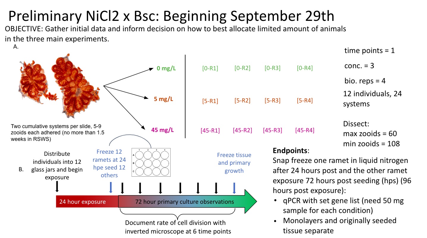
First pilot study for NiCl2 exposures on whole field-sourced Botryllus schlosseri colonies.
Objectives
Promote cell proliferation in vitro through the induction of clastogenic damage of epithelial cells derived from B. schlosseri.
If no changes are observed across the different treatments in this pilot study, identify the ideal sample size, identify manipulations to the independent variables, time or concentration of NiCl2.
Research Questions
Does an in vivo exposure to NiCl2 promote in vitro cellular proliferation of epithelial tissue subsequently seeded post exposure?
What is the rate of cell division that occurs within those first 24 hours?
How does exposure to nickel chloride impact gene expression in epithelial tissue across the different concentrations after 24 hours post exposure in vivo?
Suggestions for Experimental Design
Dr. Gardell’s suggested modifications to design 09/01/23:
Log distribution of the concentrations.
qPCR should be left for follow up experiment with better defined (targeted) concentrations and time points. Do not snap freeze tissue for qPCR, alternatively use tissue for:
Primary epithelial cell culturing to address question regarding stress-induced evolution
Use for comet assay
Valerie (UCD) Suggestions 09/23/23:
Seed tissue immediately after dissection to avoid lag time in TCM aliquot.
Reduce scale for preliminary trial to avoid 9 hours of micro-dissection time.
Final Experimental Schematic
Notes and considerations
Will not control for blastogenic stage at this time.
If system is in C2 - D blastogenic stages, seed the primary buds
If system is in A1-C1 stages, seed the parental zooids
Tissue seeding density
5-9 zooids (one whole system) in one well.
Using well plates, however, we will need to control for evaporation more effectively, currently randomly lose anywhere from 30-50% of the media, drastically causing differences in the osmolarity of the wells.
Improve humidity conditions
Add a lot of media from initiation. 2 mL in each well.
Ideal to measure media quality.
Randomize well assignments
Could be interesting to incorporate in future design, freezing tissue at the end of the exposure and then freezing after seeding. Evaluating differences in gene expression across those time points.
Experimental Planning
Animal Handling Prior to Exposure
Divided animals into separate system, 3 days prior to start of exposure, 8 days acclimated to the recirculating system.
Randomize Treatment and Plate Assignments
Here we will have R randomly assign each animal to a treatment and each treatment/animal to a different well on the plate. The idea here is to randomize placements as there may be variations in the well design.
All handling of stock solution and treatments to be done in a chemical fume hood. Once spiked water has been distributed, add animals, parafilm jars, place in secondary container, and move to environmental chamber.
Required Volume of Artificial Seawater
Calculations for spiking artificial seawater. 225 mL of seawater required to mostly submerge glass slide in wide mouth 16 oz Kerr mason jar.
Considerations:
4 replicates
225 mL per jar
3 conditions
Account for 10% loss of water during transferring
\[(4*225 * 3) + (0.1*(4*225*3)) = 2,970\]
Need 2,970 mL of artificial seawater total for exposure, particularly, 990 mL of artificial seawater per condition.
Calculations
Stock solution of NiCl2 made by undergraduate Gina Jones on 02/08/23.
NiCl2
Suspended in MilliQ water (0 PPT)
Low Dose: 5 mg/L
\[ C_1*V_1 = C_2*V_2\]\[ 1 g/L * V_1 = 0.005g/L*0.99L\]\[V_1 = 0.00495 L = 4.95 mL\] Spike 990 mL of aerated, artificial seawater (16 C) with 4.95 mL of stock NiCl2 solution. Change in salinity negligible (+/- 1 PPT).
High Dose: 45 mg/L
\[ C_1*V_1 = C_2*V_2\]\[ 1 g/L * V_1 = 0.045g/L*0.99L\]\[V_1 = 0.04455 L = 44.55 mL\] Spike 990 mL of aerated, artificial seawater (16 C) with 44.55 mL of stock NiCl2 solution. Change in salinity negligible (+/- 1 PPT).
Protocol
Subdivide animals 3 days prior to exposure start.
Make sufficient volume of artificial seawater at appropriate salinity, 25 PPT, to match recirculating seawater system parameters. In this case for a 3 x 4 exposure at 250 mL, will require about 7 L of artificial seawater.
30.8 g / L of Red Sea Salt
Rinse all glassware to be used during exposure as follows:
Triplicate rinse with lab detergent
Triplicate rinse with tap water
Triplicate rinse with DI water
Add lab bench paper to environmental chambers top rack to reduce light intensity. Include 4 slits in bench paper to allow for air flow.
Add 1000 mL of artificial seawater to three 1 L beakers and place in environmental chamber (set to ambient 23 C to achieve 16 C for water) with gentle aeration (targeting ~ 67 % DO) in preparation the night before exposure.
Day of Exposure Commencement
Take 10 mL from each 1 L beaker and document temperature, DO, pH, salinity, and ammonia of artificial seawater prior to spiking the water.
In a chemical fume hood add the appropriate volume to achieve desired concentration of nickel chloride concentration to each of the 1 L beakers using a 25 mL or 50 mL serological pipette. Be sure to homogenize solution well with the serological pipette. Distribute 225 mL of each stock to the appropriate mason jar or beaker using designated serological pipette.
Transfer animals to a portable container with artificial seawater from the recirculating system. Image the animals using the Excelis stereomicroscope. Use a razor blade to clean around the animal and to clean glass slide of excess algae and debris.
Document stage, zooid number, cumulative system number.
Distribute animals to appropriate jar in fume hood.
Parafilm jar and place in secondary container.
Transfer secondary container with jars to second rack of environmental chamber.
Leave animals for 24 hours.
Day of Dissections
Order of Takedown:
5-R3
45-R4
5-R2
0-R3
5-R4
45-R3
45-R1
5-R1
0-R2
0-R4
45-R2
0-R1
The following steps should be conducted in a chemical fume hood and iterated through one beaker at a time to avoid desiccation stress:
Remove 100% of the exposure water from beaker and dispose of NiCl2 dosed artificial seawater in the appropriately marked hazardous waste container.
With the animal and glass slide still in the beaker, quadruplicate rinse the glass slide and animal with deionized water.
Glass slide may now be handled with nitrile gloves and should be quadruplicate rinsed with artificial seawater over exposure beaker.
Transfer glass slide and animal to a fresh 16 oz mason jar containing 200 mL of 15 C artificial seawater.
Dispose of excess liquid in exposure beaker in appropriately labeled hazardous waste container.
You may now work outside the chemical fumehood. Note there may be residual NiCl2 in animal so continue to wear the appropriate PPE and work carefully.
Using a stainless steel razor blade, remove one of the two cumulative systems on the glass slide. Use forceps to transfer cumulative system to appropriately labeled snap cap 1.5 mL eppendorf PCR safe tube containing 500 uL of RNAProtect by Qiagen.
Proceed with dissection of the primary buds or zooids of the second cumulative system on the slide. Refer to epithelial isolation protocol
However, avoid using any ethanol in this procedure.
Once tissue has been removed, take cell strainer and rinse it with 30 mL ASW-PSA.
Place tissue in aliquot of TCM and immediately go to seed tissue in biosaftey cabinet. Mark time of seeding.
No replacement of media over course of trial.
Transfer samples containing cumulative system suspended in RNAProtect to -20 C freezer overnight. The following day, transfer samples to -80 C freezer for long term storage.
Data
Morphometric Records
Make sure you have made your Google sheet publicly available to anyone that has the link. If you make any updates to the sheet just re-curl the data, meaning just re-run the code below.
morph$date <-mdy(morph$date) #convert the date column from characters to true datemorph <- morph %>%separate(jar_id, c("treatment_mg_per_L", "replicate"), sep ="-") #create two new columns, treatment and replicate from jar id morph_fact <- morph %>%mutate(treatment_mg_per_L =as.factor(treatment_mg_per_L)) %>%mutate(stage =as.factor(stage)) %>%mutate(animal_id =as.factor(animal_id)) %>%mutate(date =as.factor(date)) %>%mutate(treatment_order =factor(paste(treatment_mg_per_L, animal_id))) # Create a new variable for ordering by treatment
summary(morph_fact)
   experiment            date      initials         stage        hpe
 Min.   :1.100   2023-09-29:12   Length:46          A1: 2   Min.   : 0
 1st Qu.:1.100   2023-09-30:12   Class :character   A2: 2   1st Qu.: 0
 Median :1.100   2023-10-24:11   Mode  :character   B1: 7   Median :12
 Mean   :1.148   2023-10-25:11                      B2: 6   Mean   :12
 3rd Qu.:1.200                                      C1:10   3rd Qu.:24
 Max.   :1.200                                      C2:11   Max.   :24
                                                    TO: 8
 treatment_mg_per_L  replicate            animal_id      no_sys
 0 :16              Length:46          S147C001: 2   Min.   :1.000
 45:14              Class :character   S148C001: 2   1st Qu.:1.000
 5 :16              Mode  :character   S149C001: 2   Median :1.000
                                       S151C001: 2   Mean   :1.478
                                       S154C001: 2   3rd Qu.:2.000
                                       S158C001: 2   Max.   :2.000
                                       (Other) :34
  no_prim_sys1     no_prim_sys2     image             comments
 Min.   : 4.000   Min.   : 0.0   Length:46          Length:46
 1st Qu.: 7.250   1st Qu.: 0.0   Class :character   Class :character
 Median : 8.000   Median : 7.0   Mode  :character   Mode  :character
 Mean   : 9.978   Mean   : 6.2
 3rd Qu.:12.000   3rd Qu.: 9.5
 Max.   :22.000   Max.   :19.0
                  NA's   :11
   treatment_order
 0 S148C001: 2
 0 S149C001: 2
 0 S154C001: 2
 0 S177C001: 2
 0 S209C001: 2
 0 S212C001: 2
 (Other)   :34
Exploratory plots
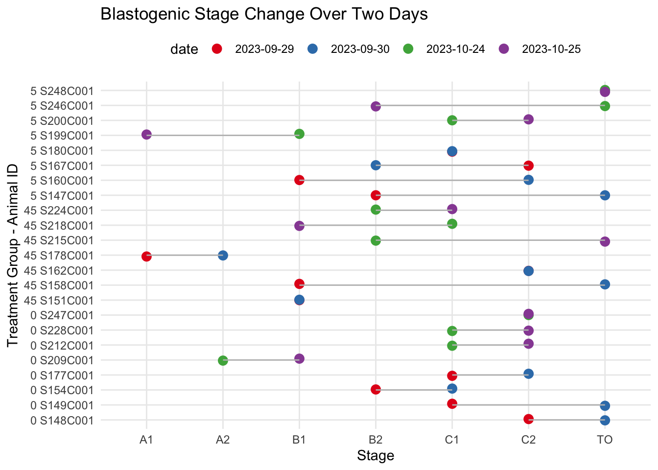
Lollipop chart to visualize the jumps or arrests in blastogenic stage progression for each animal.
# Create the plotggplot(data = morph_fact, aes(x = stage, y = treatment_order, color = date)) +geom_point(size =3, position =position_jitter(h =0.1, w =0)) +geom_line(aes(group = treatment_order), size =0.5, color ='grey') +labs(title ="Blastogenic Stage Change Over Two Days",x ="Stage", y ="Treatment Group - Animal ID") +scale_color_brewer(palette ="Set1") +theme_minimal() +theme(legend.position ="top")
Warning: Using `size` aesthetic for lines was deprecated in ggplot2 3.4.0.
ℹ Please use `linewidth` instead.
Analyzing differences in blastogenic progression across treatments
Since all the animals start at different blastogenic stages, we will need to quantify changes in blastogenic rate with a numeric scale
# Define a numeric scaleblastogenic_scale <-c("A1", "A2", "B1", "B2", "C1", "C2", "TO")numeric_scale <-1:7# Create a new variable with the numeric scalemorph <- morph %>%mutate(stage_numeric =as.integer(factor(stage, levels = blastogenic_scale, labels = numeric_scale)))
summary(morph)
   experiment         date              initials            stage
 Min.   :1.100   Min.   :2023-09-29   Length:46          Length:46
 1st Qu.:1.100   1st Qu.:2023-09-29   Class :character   Class :character
 Median :1.100   Median :2023-09-30   Mode  :character   Mode  :character
 Mean   :1.148   Mean   :2023-10-11
 3rd Qu.:1.200   3rd Qu.:2023-10-24
 Max.   :1.200   Max.   :2023-10-25

      hpe     treatment_mg_per_L  replicate          animal_id
 Min.   : 0   Length:46          Length:46          Length:46
 1st Qu.: 0   Class :character   Class :character   Class :character
 Median :12   Mode  :character   Mode  :character   Mode  :character
 Mean   :12
 3rd Qu.:24
 Max.   :24

     no_sys       no_prim_sys1     no_prim_sys2     image
 Min.   :1.000   Min.   : 4.000   Min.   : 0.0   Length:46
 1st Qu.:1.000   1st Qu.: 7.250   1st Qu.: 0.0   Class :character
 Median :1.000   Median : 8.000   Median : 7.0   Mode  :character
 Mean   :1.478   Mean   : 9.978   Mean   : 6.2
 3rd Qu.:2.000   3rd Qu.:12.000   3rd Qu.: 9.5
 Max.   :2.000   Max.   :22.000   Max.   :19.0
                                  NA's   :11
   comments         stage_numeric
 Length:46          Min.   :1.000
 Class :character   1st Qu.:4.000
 Mode  :character   Median :5.000
                    Mean   :4.848
                    3rd Qu.:6.000
                    Max.   :7.000
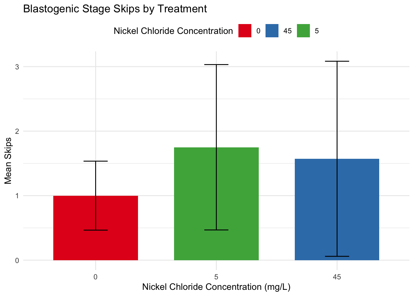
library(dplyr)# Group by treatment and animal_id, then count stage skipsskips_data <- morph %>%group_by(treatment_mg_per_L, animal_id) %>%summarize(skips =max(stage_numeric) -min(stage_numeric))
`summarise()` has grouped output by 'treatment_mg_per_L'. You can override
using the `.groups` argument.
library(ggplot2)# Calculate standard deviations for each treatmentstd_dev <- skips_data %>%group_by(treatment_mg_per_L) %>%summarize(std_dev =sd(skips))# Calculate means for each treatmentmeans_data <- skips_data %>%group_by(treatment_mg_per_L) %>%summarize(mean_skips =mean(skips))combined_data <-left_join(std_dev, means_data, by ="treatment_mg_per_L")print(combined_data)