For this weeks lab session we did a Tidy Tuesday exercise. I did the exercise using base R instead of tidyverse.
Read in the data:
library(dplyr)
library(tidyverse)

feederwatch <- readr::read_csv('https://raw.githubusercontent.com/rfordatascience/tidytuesday/master/data/2023/2023-01-10/PFW_2021_public.csv')
site_data <- readr::read_csv('https://raw.githubusercontent.com/rfordatascience/tidytuesday/master/data/2023/2023-01-10/PFW_count_site_data_public_2021.csv')
Take a look at it:
head(feederwatch)
head(site_data)
I wanted to “reduce the clutter” since I just wanted to look at Blue Jay count over the months and snow depth.
feederwatchClean <- feederwatch[,c(1,12,13,8, 21)]

sitedataClean <- site_data[,c(1, 30,31)]
Joining the data frames:
birdObs <- merge(feederwatchClean, sitedataClean)

#removing NA's
birdObs2 <- na.omit(birdObs)
Making a subset of the data:
blujayRows <- grep("blujay", birdObs2$species_code)
blueJayData <- birdObs2[blujayRows, ]
Making my plot:
par(mar = c (5, 4, 4, 4) + 0.3)
plot(type = "h", x = blueJayData$Month, y = blueJayData$how_many,
     xlab = "Month",
     ylab = "Blue Jay Count",
     main = "Change in  Blue Jay count over time and snow depth.",
     lwd = 10, col = "dark blue"
     )
par(new = TRUE) #allows us to add a new plot to overlay
plot(x = blueJayData$Month, y = blueJayData$snow_dep_atleast,
     pch = 13, col = "green",
     axes = FALSE,
     xlab = "", ylab = "")
axis(side = 4, at = pretty(range(blueJayData$snow_dep_atleast)))
mtext("Pecieved snow depth (inches)", side = 4, line = 2)
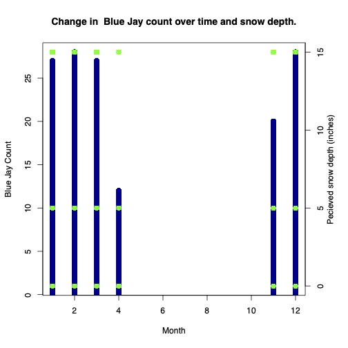
In retrospect I don’t think I properly cleaned my data to visualize the question I had.